
We showed in the last post what tensors are, what the ‘flow’ means, and how they are represented in TensorFlow. Here, we’ll do something much more exciting.
Let’s go through a simple example where we’ll use TensorFlow to find the Circumference of any circle given the radius.
We already know that the formula for finding the circumference of a
circle with it’s radius is $C = 2πr$,
where $C = circumference, r = radius, π = 3.14$
But our tensorflow model doesn’t know that rule, and we want it to find it’s own rule for correctly calculating circumferences.
We’ll do this by allowing our tensorflow model to go through some set of radius values and their corresponding circumference values and try to find out the relationship between them.
Here’s our sample dataset:
radius_values = [2.0, 4.0, 8.0, 7.0, 6.0, 5.0, 1.0, 11.0, 3.0, 5.0, 4.0, 2.0] circumference_values = [12.57, 25.13, 50.27, 43.98, 37.70, 31.42, 6.28, 69.12, 18.85, 31.42, 25.13, 12.57]
Before we commence, it is important to already notice that this case is perfect for representing a simple linear regression.
What is Linear Regression?
The idea of Linear Regression in machine learning is about the task of predicting a continuous quantity which is always a numerical value.
Regression establishes a relationship between a dependent variable Y and one or more independent variables X, using a best fit straight line (also known as regression line).
In Linear Regression, when the independent variable is single, it is described as a Simple Linear Regression, whereas cases where the independent variables are more than one are described as Multiple Linear Regression.
Import dependencies
First, we’ll import TensorFlow as well as NumPy to help us represent our data
import tensorflow as tf
import numpy as np
Provide the data
Next, we create two lists radius_values and circumference_values that
hold the set of data to be used to train our model.
radius_values         = np.array([2.0, 4.0, 8.0, 7.0, 6.0, 5.0, 1.0, 11.0, 3.0, 5.0, 4.0, 2.0],  dtype=float)
circumference_values  = np.array([12.57, 25.13, 50.27, 43.98, 37.70, 31.42, 6.28, 69.12, 18.85, 31.42, 25.13, 12.57],  dtype=float)

for i, r in enumerate(radius_values):
  print("Given radius to be = {}, the Circumference = {}".format(r, circumference_values[i]))
which prints:
Given radius to be = 2.0, the Circumference = 12.57
Given radius to be = 4.0, the Circumference = 25.13
Given radius to be = 8.0, the Circumference = 50.27
Given radius to be = 7.0, the Circumference = 43.98
Given radius to be = 6.0, the Circumference = 37.7
Given radius to be = 5.0, the Circumference = 31.42
Given radius to be = 1.0, the Circumference = 6.28
Given radius to be = 11.0, the Circumference = 69.12
Given radius to be = 3.0, the Circumference = 18.85
Given radius to be = 5.0, the Circumference = 31.42
Given radius to be = 4.0, the Circumference = 25.13
Given radius to be = 2.0, the Circumference = 12.57
Create the model — a simple neural network that represents a linear regression
Next, we will create the simplest possible neural network. Since the problem is straightforward, this network will require only a single layer, with a single neuron, with input shape as just 1 value.
model = tf.keras.Sequential([keras.layers.Dense(units=1, input_shape=[1])])Compile the model, with loss and optimizer functions
Our model has to be compiled before training. And to do compile, we must specify 2 functions, a loss and an optimizer.
Loss function is a way of measuring how far off predictions are from the desired outcome. While Optimizer function is a way of adjusting internal values in order to reduce the loss.
For the loss, we use the MEAN SQUARED ERROR, and for the optimizer, we’ll use the STOCHASTIC GRADIENT DESCENT.
model.compile(loss='mean_squared_error', optimizer='sgd')Train the model
We call model.fit to train our neural network.
This is the process where the model learns the relationship between the radius values and their corresponding circumference values.
Hence, the fit() method takes in the radius_values (as features),
the circumference_values (as labels). The epochs argument depicts how
many times the cycle would be run, while the verbose argument controls
how much output the method produces.
history = model.fit(radius_values, circumference_values, epochs=500, verbose=False)
print("Finished training the model")
Plot training statistics
The history object that we assigned to the fit method
can be used to plot the loss of our model.
Let’s use Matplotlib to visualize the gradient of the loss.
import matplotlib.pyplot as plt

plt.xlabel('Epoch Number')
plt.ylabel("Loss Magnitude")
plt.plot(history.history['loss'])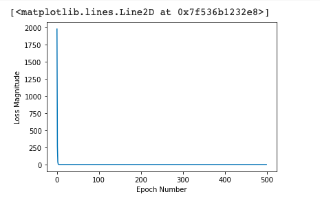
Predict new values with our model
Let’s now pick a random number for radius and ask our model to predict it’s circumference.
We’ll try 10.0
print(model.predict([10.0]))The result 62.8 looks really good.
The correct answer is 2 × 3.14 × 10.0 = 62.83 , so our model is doing really well.
Our model can now correctly provide the circumference of any circle, given it’s radius.
See the entire colab notebook here.