
Continued from part one, where we’ve completed pre-processing (cleaning, formatting, etc) the dataset. Let’s now go ahead to build our TensorFlow model to help suggest near-perfect used car prices.
Our dataset now looks really good for training the model. But before we commence training, we need to separate a set of training data from another smaller set of test data.
We also need to define the labels (Y).
Let’s go!
Splitting the dataset
Let us split the dataset into a training set and a test set. We’ll only use the test set in the final evaluation of the model.
train_dataset = dataset.sample(frac=0.8, random_state=0)
test_dataset = dataset.drop(train_dataset.index)
Inspecting the data
Next, using sns, let’s try to have a quick look at the joint distribution of a few pairs of columns from the training set.
sns.pairplot(train_dataset[["Price", "Year", "Engine", "Power"]],
    diag_kind="kde")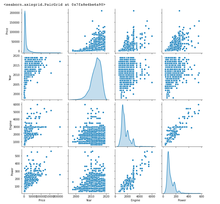
Separate the features from labels
I now separate the target value, or “label”, from the features. And check the overall statistics:
train_labels = train_dataset.pop('Price')
test_labels = test_dataset.pop('Price')
train_stats = train_dataset.describe()
train_stats = train_stats.transpose()
train_stats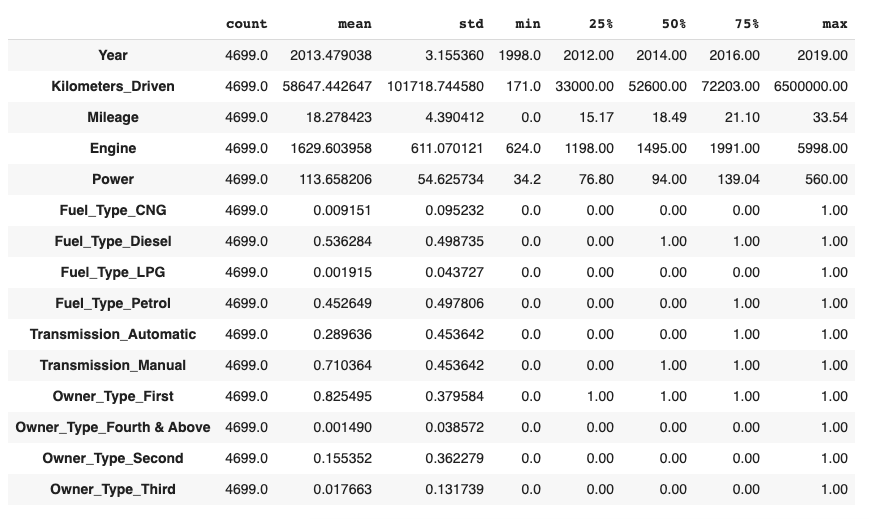
Normalize the data
A look at the statistical data above shows how widely different the ranges of each features are. To make our training easier and ensuring that our model is a lot less dependent on certain specific units rather than all of them, we’ll perform feature normalization.
def norm(x):
  return (x - train_stats['mean']) / train_stats['std']

normed_train_data = norm(train_dataset)
normed_test_data = norm(test_dataset)

normed_train_data.head()
Training our model
We’ll use a Sequential model with eight multiple connected hidden layers, and an output layer that returns a single, continuous value.
def build_model():
  model = tf.keras.Sequential([
    tf.keras.layers.Dense(256, activation='relu', input_shape=[len(train_dataset.keys())]),
    tf.keras.layers.Dense(256, activation='relu'),
    tf.keras.layers.Dense(256, activation='relu'),
    tf.keras.layers.Dense(128, activation='relu'),
    tf.keras.layers.Dense(128, activation='relu'),
    tf.keras.layers.Dense(128, activation='relu'),
    tf.keras.layers.Dense(64, activation='relu'),
    tf.keras.layers.Dense(64, activation='relu'),
    tf.keras.layers.Dense(1)
  ])

  optimizer = tf.keras.optimizers.RMSprop(0.001)

  model.compile(loss='mse',
                optimizer=optimizer,
                metrics=['mae', 'mse'])
  return model
Build the model and view the summary
model = build_model()
model.summary()
Let’s now train the model for 1000 epochs, and record the training and validation accuracy in ‘history’.
EPOCHS = 1000

history = model.fit(
  normed_train_data, train_labels,
  epochs=EPOCHS, validation_split = 0.2, verbose=0,
  callbacks=[tfdocs.modeling.EpochDots()])
Let’s now visualize the model’s training progress using the stats stored in the history object.
plotter = tfdocs.plots.HistoryPlotter(smoothing_std=2)Using the MAE (Mean Absolute Error)
plotter.plot({'Basic': history}, metric = "mae")
plt.ylim([0, 5000])
plt.ylabel('MAE [Price]')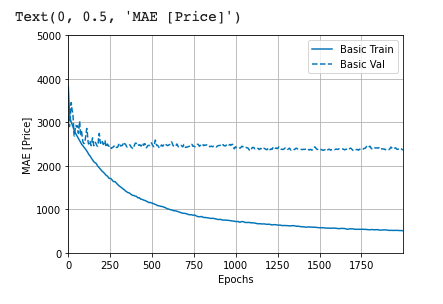
Testing our model
Let’s take a single batch from our normalised test data and predict the price
example_batch = normed_test_data[5:6]
example_batch

example_result = model.predict(example_batch)
print(example_result)
We get [[8259.985]], which means about 8,260 in USD
Let’s draw a prediction graph of our entire test data with our regression model
test_predictions = model.predict(normed_test_data).flatten()

a = plt.axes(aspect='equal')
plt.scatter(test_labels, test_predictions)
plt.xlabel('True Values [Price]')
plt.ylabel('Predictions [Price]')
lims = [0, 100000]
plt.xlim(lims)
plt.ylim(lims)
_ = plt.plot(lims, lims)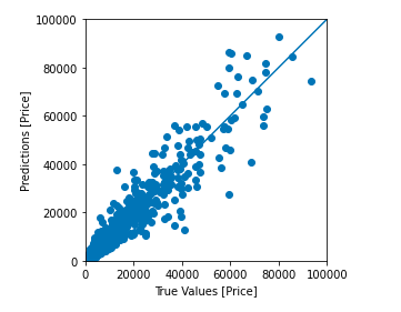
And finally, we can take a look at it’s error distribution:
error = test_predictions - test_labels
plt.hist(error, bins = 25)
plt.xlabel("Prediction Error [Price]")
_ = plt.ylabel("Count")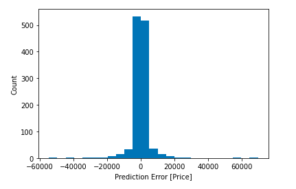
That does it. See the full Colab notebook here.