
You’ve got a used car you’d like to sell. You know the acquired price, but how do you measure how much a fair sale price would be based on how much it has been used?
Let’s build a TensorFlow model to help suggest near-perfect used car prices.
This post is a step by step approach to how I built suggestcarprice.xyz
Now, we already established in a previous post that the idea of Linear Regression in machine learning is about the task of predicting a continuous quantity which is always a numerical value.
And that while Regression in itself establishes a relationship between a dependent variable Y and one or more independent variables X, it is important to realise that in Linear Regression, when the independent variable is single, it is described as a Simple Linear Regression, whereas cases where the independent variables are more than one are described as Multiple Linear Regression.
And since we’ll be dealing with multiple car qualities that would make up what a likely price would be, our machine learning model approach would be perfectly described as Multiple Linear Regression.
Let’s now describe the dataset to be used.
I make use of a pretty handy used cars dataset from @avikasliwal on Kaggle ( kaggle.com/avikasliwal/used-cars-price-prediction), and it’s got the following columns:
- Name: The brand and model of the car
- Location: The location in which the car is being sold or is available for purchase
- Year: The year or edition of the model
- Kilometers_Driven: The total kilometres driven in the car by the previous owner(s) in KM
- Fuel_Type: The type of fuel used by the car (Petrol, Diesel, Electric, CNG, LPG)
- Transmission: The type of transmission used by the car (Automatic / Manual)
- Owner_Type: Position of ownership at that time
- Mileage: The standard mileage offered by the car company in kmpl or km/kg
- Engine: The displacement volume
Already downloaded the dataset? Let’s start coding!
First, we import the necessary libraries
import numpy as np
import pandas as pd
import matplotlib.pyplot as plt
import seaborn as sns

import tensorflow as tf

import tensorflow_docs as tfdocs
import tensorflow_docs.plots
import tensorflow_docs.modeling
The dataset is a CSV file named “cars-train-data.csv”. Let’s define the columns, import it in using Pandas, and start cleaning it.
column_names = ['Ind', 'Name', 'Location', 'Year', 'Kilometers_Driven',
    'Fuel_Type', 'Transmission', 'Owner_Type', 'Mileage', 'Engine',
    'Power', 'Seats', 'New_Price', 'Price']
raw_dataset = pd.read_csv(dataset_path, names=column_names,
    na_values = "?", comment='\t', skiprows=1, sep=",",
    skipinitialspace=True)

dataset = raw_dataset.copy()
dataset.head()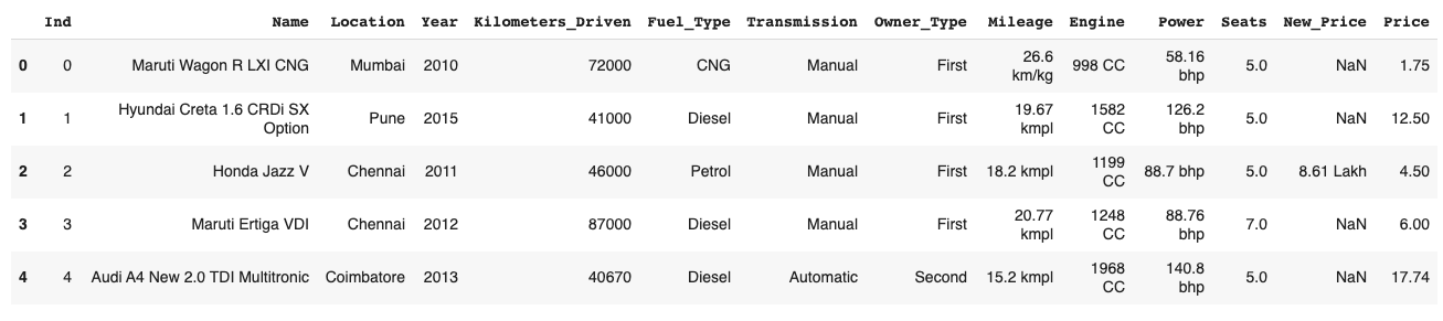
Next, let’s drop the columns we would not need
dataset = dataset.drop(columns=['Ind', 'Name', 'Location', 'Seats',
    'New_Price'])
dataset.head()
Then, to see a good description of the dataset
dataset.describe()Cleaning the data
The dataset contains a few unknown values. Let’s find them and drop them.
dataset.isna().sum()
dataset = dataset.dropna()
dataset = dataset.reset_index(drop=True)

dataset.head()
Next, let’s format our samples. We’ll use regular expression to remove non-numeric characters like “km/kg”, “CC”, “bhp”, etc, from the following columns
import re

dataset['Mileage'] = pd.Series([re.sub('[^.0-9]', '',
    str(val)) for val in dataset['Mileage']], index = dataset.index)
dataset['Engine'] = pd.Series([re.sub('[^.0-9]', '',
    str(val)) for val in dataset['Engine']], index = dataset.index)
dataset['Power'] = pd.Series([re.sub('[^.0-9]', '',
    str(val)) for val in dataset['Power']], index = dataset.index)
The prices are by default in INR Lakhs. So, we have to convert them to USD
dataset['Price'] = pd.Series([int(float(val)*1317.64)
    for val in dataset['Price']], index = dataset.index)
After that formatting, it turns out there are some whitespaces (empty strings with one space in-between) in our dataset that are very sure to affect our training. Let’s reformat every whitespace to np.nan values, so that we can then recognise them and delete them.
dataset = dataset.replace(r'^\s*$', np.nan, regex=True)
dataset.isna().sum()
dataset = dataset.dropna()

dataset = dataset.reset_index(drop=True)
dataset.head()
Next, we’ll convert the strings in the below columns into float values. Remember that we can only work with numerical values.
dataset['Mileage'] = pd.Series([float(str(val))
    for val in dataset['Mileage']], index = dataset.index)
dataset['Engine'] = pd.Series([float(str(val))
    for val in dataset['Engine']], index = dataset.index)
dataset['Power'] = pd.Series([float(val)
    for val in dataset['Power']], index = dataset.index)
Now, let’s re-arrange the columns. I do this to have a better view of the features in an order of visual priority (so to say). Also, to put the label (the label is the value Y we’re trying to predict, and in this case, it is the Price) before the rest of the columns.
dataset = dataset[['Price', 'Year', 'Kilometers_Driven',
    'Mileage', 'Engine', 'Power', 'Owner_Type', 'Transmission',
    'Fuel_Type']]
dataset.head()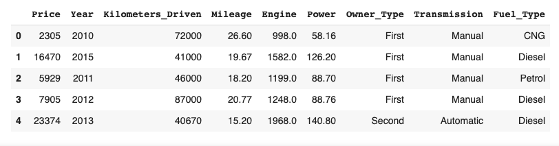
Notice how that last three columns (Owner_Type, Transmission, Fuel_Type) are not numerical values, but categorical entries?
To utilise the columns, we’ll need to find a way to make them numerical, and a perfect technique is One-hot Encoding (read my previously written post about one-hot encoding here).
Let’s now one-hot encode these columns.
Fuel_Type column:
print(dataset['Fuel_Type'].unique())
dataset['Fuel_Type'] = pd.Categorical(dataset['Fuel_Type'])
dfFuel_Type = pd.get_dummies(dataset['Fuel_Type'], prefix = 'Fuel_Type')
dfFuel_Type.head()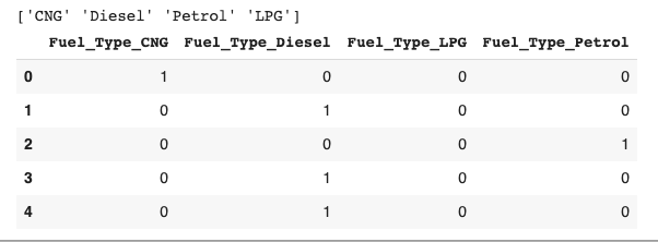
Transmission column:
print(dataset['Transmission'].unique())
dataset['Transmission'] = pd.Categorical(dataset['Transmission'])
dfTransmission = pd.get_dummies(dataset['Transmission'], prefix = 'Transmission')
dfTransmission.head()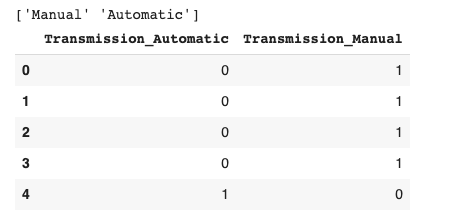
Owner_Type column:
print(dataset['Owner_Type'].unique())
dataset['Owner_Type'] = pd.Categorical(dataset['Owner_Type'])
dfOwner_Type = pd.get_dummies(dataset['Owner_Type'], prefix = 'Owner_Type')
dfOwner_Type.head()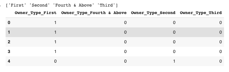
Let’s now concatenate all the one-hot encoded data with our dataset, and drop their original columns as we no longer need them.
dataset = pd.concat([dataset, dfFuel_Type, dfTransmission, dfOwner_Type], axis=1)
dataset = dataset.drop(columns=['Owner_Type', 'Transmission', 'Fuel_Type'])
dataset.head()
Let’s stop here for now. In the next post, we’ll continue with splitting our data into training and testing, normalising the values, and then train our model to help predict used car prices.
See here: Predicting Car Prices with TensorFlow — a case of Multiple Linear Regression (2 of 2)